R

Regression from linear fits to logistic and ridge models, and ggplot2 charts that state their finding.

Predicting Flight Delays

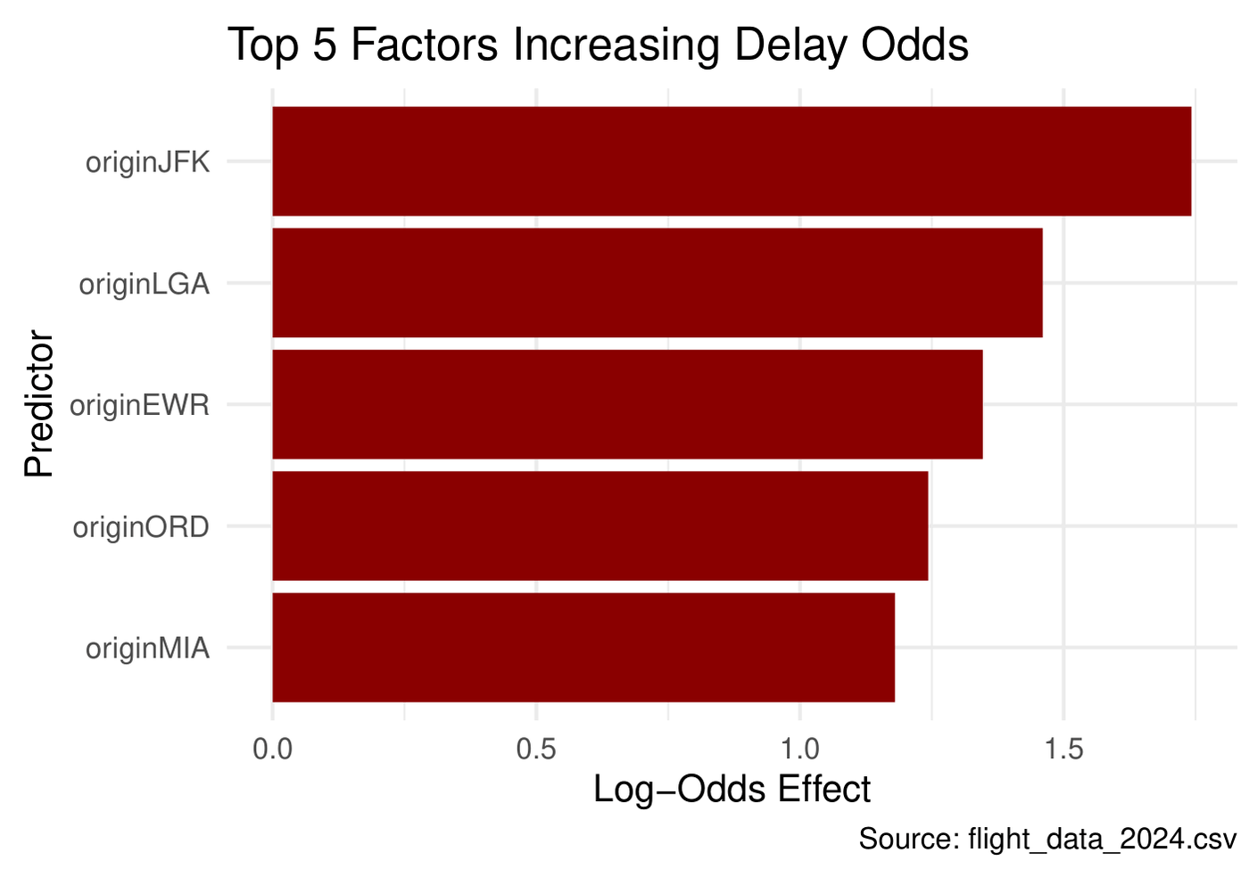
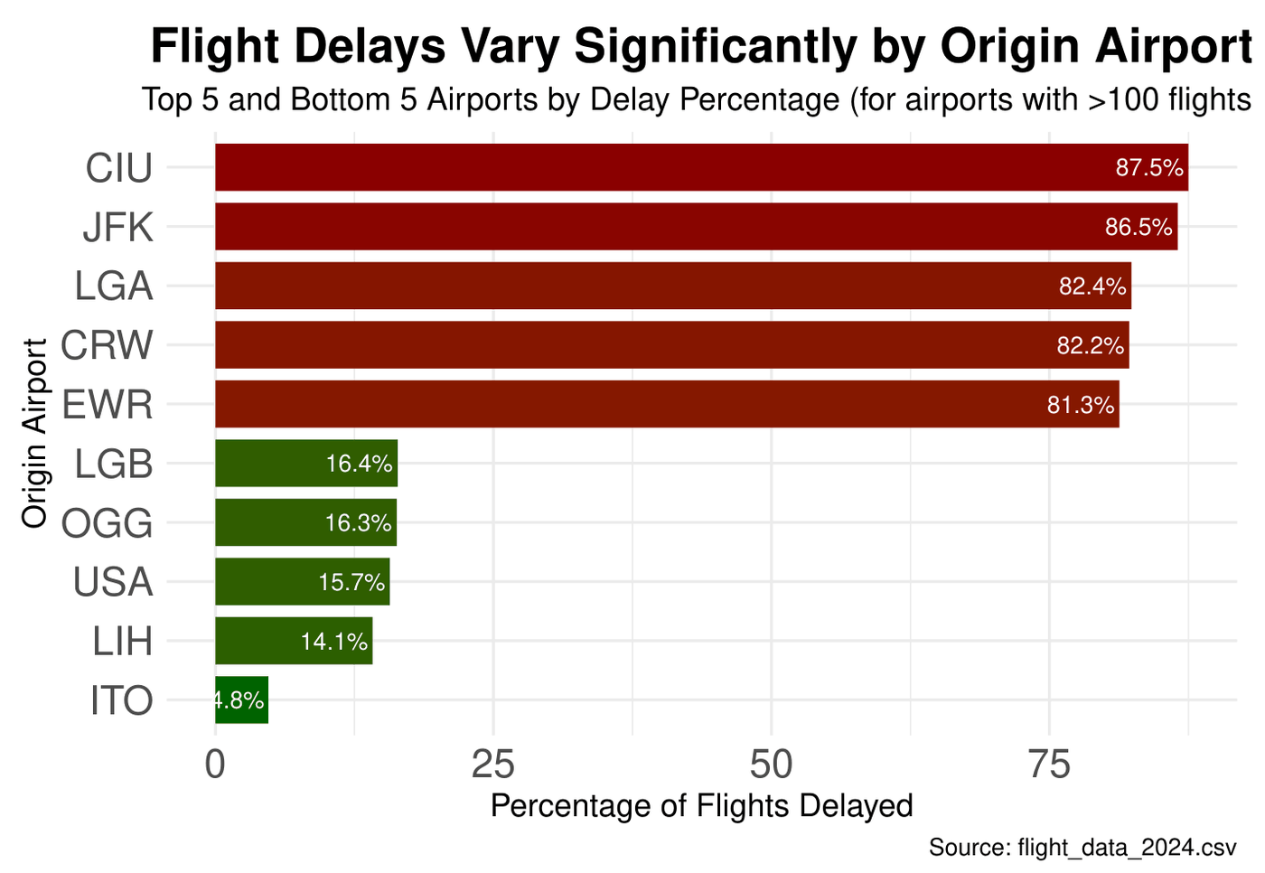
Logistic regression on over one million U.S. flights from January and February 2024. The model uses origin airport, departure time, day of week and distance, and is tested on a held-out 20%. JFK, LaGuardia and Newark add the most delay risk.

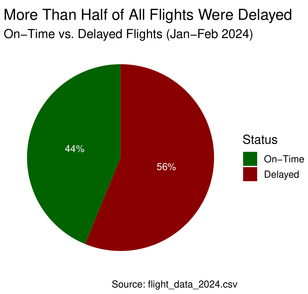
56%of flights delayed 15+ min
65.2%accuracy vs 56.2% baseline
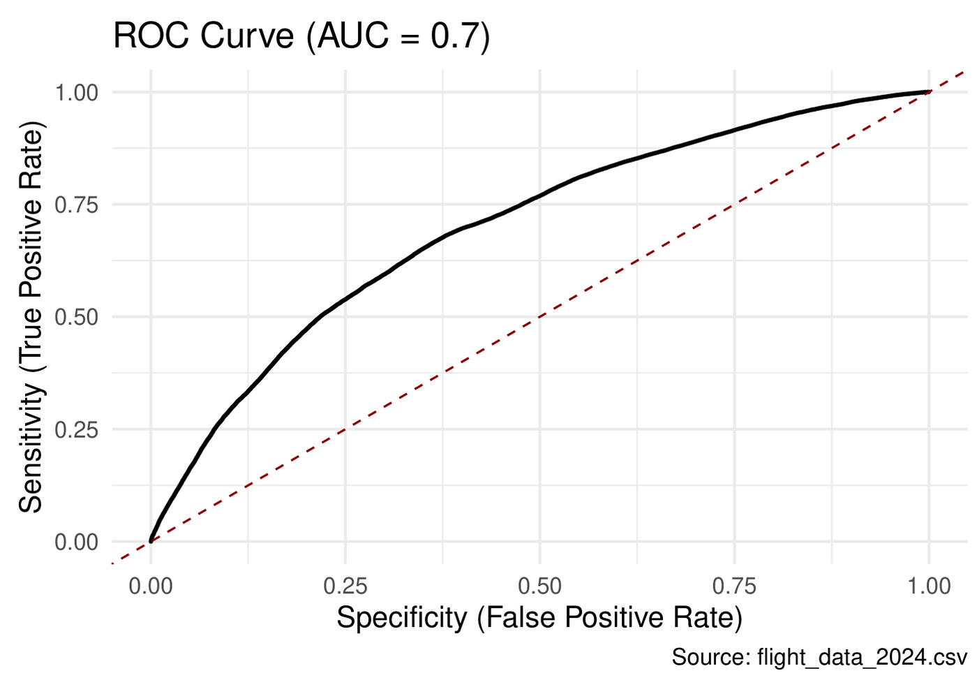
0.70ROC AUC
glm binomialcaretpROCbroomggplot2
Full write-up (PDF)
Top and bottom five origin airports by share of flights delayedTop five factors increasing delay odds: JFK, LGA, EWR, ORD, MIAROC curve, AUC 0.756 percent of flights delayed
Code · 192 lines
# Predicting Flight Delays: A Logistic Regression Approach
#
# Question: can we predict the likelihood of a flight delay from its origin
# airport, scheduled departure time, day of the week and flight distance?
# Data: over one million U.S. flights, January-February 2024 (BTS on-time data).
# A flight counts as "delayed" when wheels-off is 15+ minutes after scheduled departure.

library(tidyverse)
library(pROC)
library(caret)
library(broom)

# 1.0 Load and profile ----
flight_data_raw <- read_csv("flight_data_2024.csv")
glimpse(flight_data_raw)

sum(is.na(flight_data_raw))
(sum(is.na(flight_data_raw)) / (nrow(flight_data_raw) * ncol(flight_data_raw))) * 100

# 2.0 Clean ----
# Drop cancelled flights and delays caused by weather or a late inbound aircraft,
# so the model only sees delays the airport and schedule could explain.
airplane_data <- flight_data_raw %>%
  filter(cancelled == 0,
         weather_delay == 0,
         late_aircraft_delay == 0,
         !is.na(dep_time),   # model uses this
         !is.na(taxi_out)    # model uses this
         ) %>%
  select(-air_time, -taxi_in, -late_aircraft_delay, -weather_delay,
         -cancelled, -origin_city_name, -origin_state_nm, -month,
         -day_of_month, -wheels_on, -year)

removed_rows <- nrow(flight_data_raw) - nrow(airplane_data)
paste(removed_rows, "flights removed.")

# 3.0 Build the target ----
# HHMM integers -> real datetimes; a wheels-off time earlier than departure
# means the flight crossed midnight, so add a day.
airplane_data <- airplane_data %>%
  mutate(
    dep_time_str = sprintf("%02d:%02d", dep_time %/% 100, dep_time %% 100),
    wheels_off_str = sprintf("%02d:%02d", wheels_off %/% 100, wheels_off %% 100),
    dep_datetime = mdy_hm(paste(fl_date, dep_time_str)),
    wheels_off_datetime = mdy_hm(paste(fl_date, wheels_off_str)),
    wheels_off_datetime = if_else(wheels_off_datetime < dep_datetime,
                                  wheels_off_datetime + days(1), wheels_off_datetime),
    delay_time = as.numeric(difftime(wheels_off_datetime, dep_datetime, units = "mins")),
    delayed = ifelse(delay_time >= 15, 1, 0),
    day = factor(day_of_week, levels = 1:7,
                 labels = c("Monday", "Tuesday", "Wednesday", "Thursday",
                            "Friday", "Saturday", "Sunday"))
  )

# 4.0 Explore ----
delay_summary <- airplane_data %>%
  count(delayed) %>%
  mutate(prop = n / sum(n))

ggplot(delay_summary, aes(x = "", y = prop, fill = factor(delayed))) +
  geom_bar(stat = "identity", width = 1) +
  coord_polar("y", start = 0) +
  geom_text(aes(label = scales::percent(prop)), color = "white",
            position = position_stack(vjust = 0.5)) +
  scale_fill_manual(values = c("0" = "darkgreen", "1" = "darkred"),
                    labels = c("On-Time", "Delayed")) +
  labs(title = "More Than Half of All Flights Were Delayed",
       subtitle = "On-Time vs. Delayed Flights (Jan-Feb 2024)",
       fill = "Status", caption = "Source: flight_data_2024.csv") +
  theme_void(base_size = 14)

# Delay rate by origin airport (airports with 100+ flights only)
delay_by_origin <- airplane_data %>%
  group_by(origin) %>%
  summarise(total_flights = n(),
            delayed_flights = sum(delayed),
            delay_percentage = (delayed_flights / total_flights) * 100) %>%
  arrange(desc(delay_percentage)) %>%
  filter(total_flights > 100)

plot_data_origin <- bind_rows(head(delay_by_origin, 5), tail(delay_by_origin, 5)) %>%
  mutate(origin = fct_reorder(origin, delay_percentage))

ggplot(plot_data_origin, aes(x = origin, y = delay_percentage, fill = delay_percentage)) +
  geom_col(width = 0.8) +
  geom_text(aes(label = paste0(round(delay_percentage, 1), "%")),
            hjust = 1.07, size = 3, color = "white") +
  labs(title = "Flight Delays Vary Significantly by Origin Airport",
       subtitle = "Top 5 and Bottom 5 Airports by Delay Percentage (airports with >100 flights)",
       caption = "Source: flight_data_2024.csv",
       x = "Origin Airport", y = "Percentage of Flights Delayed") +
  scale_fill_gradient(low = "darkgreen", high = "darkred") +
  coord_flip() +
  theme_minimal() +
  theme(plot.title = element_text(hjust = 0.5, face = "bold", size = 18),
        plot.subtitle = element_text(hjust = 0.5, size = 12),
        axis.title = element_text(size = 12),
        axis.text = element_text(size = 15),
        legend.position = "none")

# Best and worst day of the week
delay_by_day <- airplane_data %>%
  group_by(day) %>%
  summarise(pct_delay = mean(delayed) * 100)

max_delay_by_day <- delay_by_day %>%
  slice_max(pct_delay, n = 1) %>%
  mutate(type = "Highest Delay Day")

min_delay_by_day <- delay_by_day %>%
  slice_min(pct_delay, n = 1) %>%
  mutate(type = "Lowest Delay Day")

delay_day_summary <- rbind(max_delay_by_day, min_delay_by_day)
delay_day_summary <- delay_day_summary[, c("type", "day", "pct_delay")]
colnames(delay_day_summary) <- c("Type", "Day", "Percent_Delayed")
delay_day_summary

# 5.0 Model ----
# Keep the 50 busiest airports as their own levels; group the rest as "Other"
top_50_airports <- airplane_data %>%
  count(origin, sort = TRUE) %>%
  slice_max(n, n = 50) %>%
  pull(origin)

model_data <- airplane_data %>%
  mutate(origin = ifelse(origin %in% top_50_airports, origin, "Other")) %>%
  select(delayed, origin, dep_time, distance, day) %>%
  na.omit()

model_data$origin <- as.factor(model_data$origin)
model_data$day <- as.factor(model_data$day)
model_data$day <- relevel(model_data$day, ref = "Friday")  # Friday = baseline

set.seed(123)
train_index <- createDataPartition(model_data$delayed, p = 0.8, list = FALSE)
train_data <- model_data[train_index, ]
test_data <- model_data[-train_index, ]

logit_model <- glm(delayed ~ ., data = train_data, family = "binomial")

coefs <- coef(logit_model)
sort(abs(coefs), decreasing = TRUE)[1:5]    # strongest effects
sort(abs(coefs), decreasing = FALSE)[1:5]   # weakest effects

# 6.0 Evaluate on the held-out 20% ----
predictions <- predict(logit_model, test_data, type = "response")
predicted_classes <- ifelse(predictions > 0.5, 1, 0)

conf_matrix <- confusionMatrix(factor(predicted_classes), factor(test_data$delayed))
print(conf_matrix)

roc_obj <- roc(test_data$delayed, predictions)
auc_value <- auc(roc_obj)

plot_data <- data.frame(FPR = 1 - roc_obj$specificities, TPR = roc_obj$sensitivities)

ggplot(plot_data, aes(x = FPR, y = TPR)) +
  geom_line(color = "black", size = 1) +
  geom_abline(intercept = 0, slope = 1, linetype = "dashed", color = "darkred") +
  labs(title = paste0("ROC Curve (AUC = ", round(auc_value, 2), ")"),
       x = "Specificity (False Positive Rate)",
       y = "Sensitivity (True Positive Rate)",
       caption = "Source: flight_data_2024.csv") +
  theme_minimal(base_size = 14)

# 7.0 Which factors move the odds of a delay? ----
model_summary <- tidy(logit_model) %>%
  filter(term != "(Intercept)") %>%
  mutate(odds_ratio = exp(estimate),
         variable_group = case_when(
           grepl("origin", term) ~ "Airport (Origin)",
           grepl("day", term) ~ "Day of Week",
           TRUE ~ "Numeric"))

top_pos <- model_summary %>% arrange(desc(estimate)) %>% slice(1:5)
ggplot(top_pos, aes(x = reorder(term, estimate), y = estimate)) +
  geom_col(fill = "darkred") +
  coord_flip() +
  labs(title = "Top 5 Factors Increasing Delay Odds",
       x = "Predictor", y = "Log-Odds Effect",
       caption = "Source: flight_data_2024.csv") +
  theme_minimal(base_size = 14)
top_neg <- model_summary %>% arrange(estimate) %>% slice(1:5)
ggplot(top_neg, aes(x = reorder(term, estimate), y = estimate)) +
  geom_col(fill = "darkgreen") +
  coord_flip() +
  labs(title = "Top 5 Factors Decreasing Delay Odds",
       x = "Predictor", y = "Log-Odds Effect",
       caption = "Source: flight_data_2024.csv") +
  theme_minimal(base_size = 14)
What Drives Caterpillar Sales?

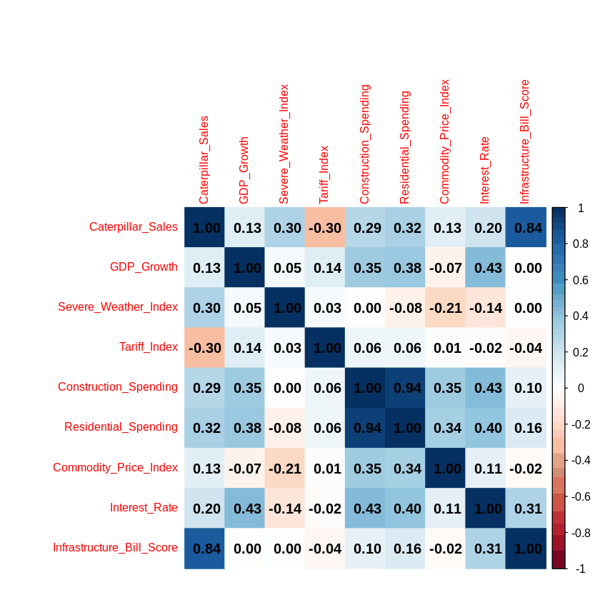
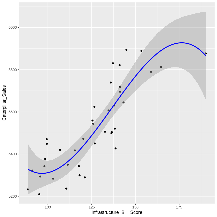
Screens eight macro indicators against 39 quarters of sales, finds the curve in the strongest driver, then drops Construction Spending (r = 0.94 with Residential, p = 0.74). The model gets simpler and better.

0.9288 → 0.9307adjusted R²
0.0701 → 7e-07Residential Spending p-value
lmcubic fitLOWESScorrplotmulticollinearity
Correlation matrix of Caterpillar sales and macro indicatorsCubic fit of sales on infrastructure bill score
Code · 80 lines
# What drives Caterpillar sales? Correlation screening, linear vs cubic fits,
# multiple regression, and removing a predictor that causes multicollinearity.
# Data: 39 quarters of Caterpillar sales with eight macro indicators.

library(ggplot2)
library(readr)
library(corrplot)

df <- read.csv("Caterpillar_TimeSeries.csv")

# 1.0 Distribution of the target (sales in millions) ----
summary(df)
summary(df$Caterpillar_Sales)
summary(df$Interest_Rate)

hist(df$Caterpillar_Sales, col = "skyblue",
     xlab = "Sales (in millions)", main = "Distribution of Sales")
boxplot(df$Caterpillar_Sales, col = "orange", main = "Boxplot of Sales")
plot(density(df$Caterpillar_Sales),
     main = "Density Plot of Sales", xlab = "Sales (in millions)")

# 2.0 Correlations ----
cor(df$Caterpillar_Sales, df$Tariff_Index)
# -0.3048: makes sense. Higher tariffs raise costs, which lowers sales.

df_numeric <- df[sapply(df, is.numeric)]   # keep numeric columns only
cor_matrix <- cor(df_numeric)
corrplot(cor_matrix, method = "color", addCoef.col = "black", tl.cex = 0.8)

# Rank every variable by the strength of its correlation with sales
sales_cor <- cor_matrix[, "Caterpillar_Sales"]
sales_df <- data.frame(Variable = names(sales_cor), Correlation = sales_cor)
top_7_corr <- sales_df[order(-abs(sales_df$Correlation)), ][1:7, ]   # target + 6 predictors
top_7_corr
# The directions make sense:
#   Infrastructure_Bill_Score up -> sales up (more funding, more machinery)
#   Residential_Spending up      -> sales up (housing projects need heavy equipment)
#   Tariff_Index up              -> sales down (less trade, higher costs)

# 3.0 Strongest single predictor: linear vs cubic ----
plot(df$Infrastructure_Bill_Score, df$Caterpillar_Sales)
abline(lm(Caterpillar_Sales ~ Infrastructure_Bill_Score, data = df), col = "red")
lines(lowess(df$Infrastructure_Bill_Score, df$Caterpillar_Sales), col = "darkgreen")
# The LOWESS line curves, so a non-linear model may fit better.

model_linear <- lm(Caterpillar_Sales ~ Infrastructure_Bill_Score, data = df)
summary(model_linear)

model_cubic <- lm(Caterpillar_Sales ~ poly(Infrastructure_Bill_Score, 3, raw = TRUE), data = df)
summary(model_cubic)
# The cubic model has the higher R-squared, so it explains more of the variance in sales.

ggplot(df, aes(x = Infrastructure_Bill_Score, y = Caterpillar_Sales)) +
  geom_point() +
  geom_smooth(method = "lm", formula = y ~ poly(x, 3), color = "blue")

# 4.0 Multiple regression with the top six predictors ----
model_multiple <- lm(Caterpillar_Sales ~ Infrastructure_Bill_Score +
  Residential_Spending + Severe_Weather_Index + Tariff_Index +
  Construction_Spending + Interest_Rate,
  data = df)
summary(model_multiple)

# 5.0 Multicollinearity check ----
corrplot(cor_matrix, method = "color", addCoef.col = "black", tl.cex = 0.8)
# Construction_Spending and Residential_Spending correlate at 0.94.
# (Infrastructure_Bill_Score vs sales doesn't count: that's target vs predictor.)
# The overlap inflates standard errors and blurs which variable drives sales.
# Construction_Spending also has p = 0.7430, far above 0.05, so it adds nothing
# unique. Remove it.

model2_multiple <- lm(Caterpillar_Sales ~ Infrastructure_Bill_Score +
  Residential_Spending + Severe_Weather_Index + Tariff_Index +
  Interest_Rate,
  data = df)
summary(model2_multiple)
# Result:
#   Adjusted R-squared rises from 0.9288 to 0.9307 with one fewer variable.
#   Residential_Spending goes from p = 0.0701 (not significant) to p = 7.33e-07.
#   With Construction_Spending gone, multicollinearity is no longer a concern.

Ames Housing: EDA to Ridge Regression

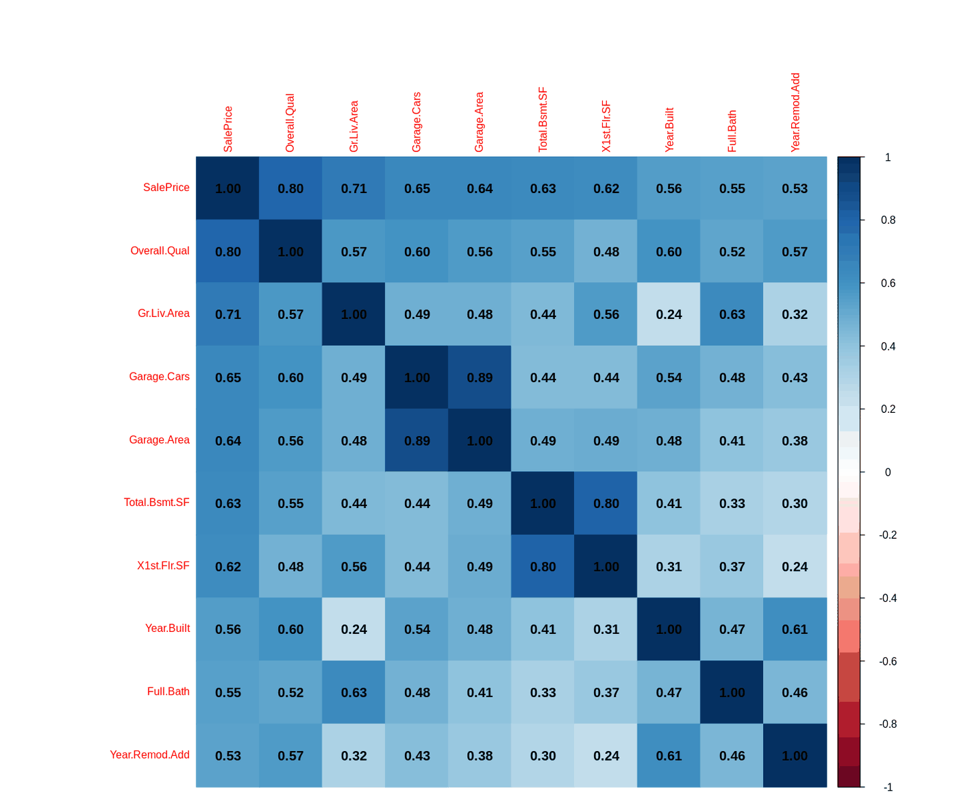
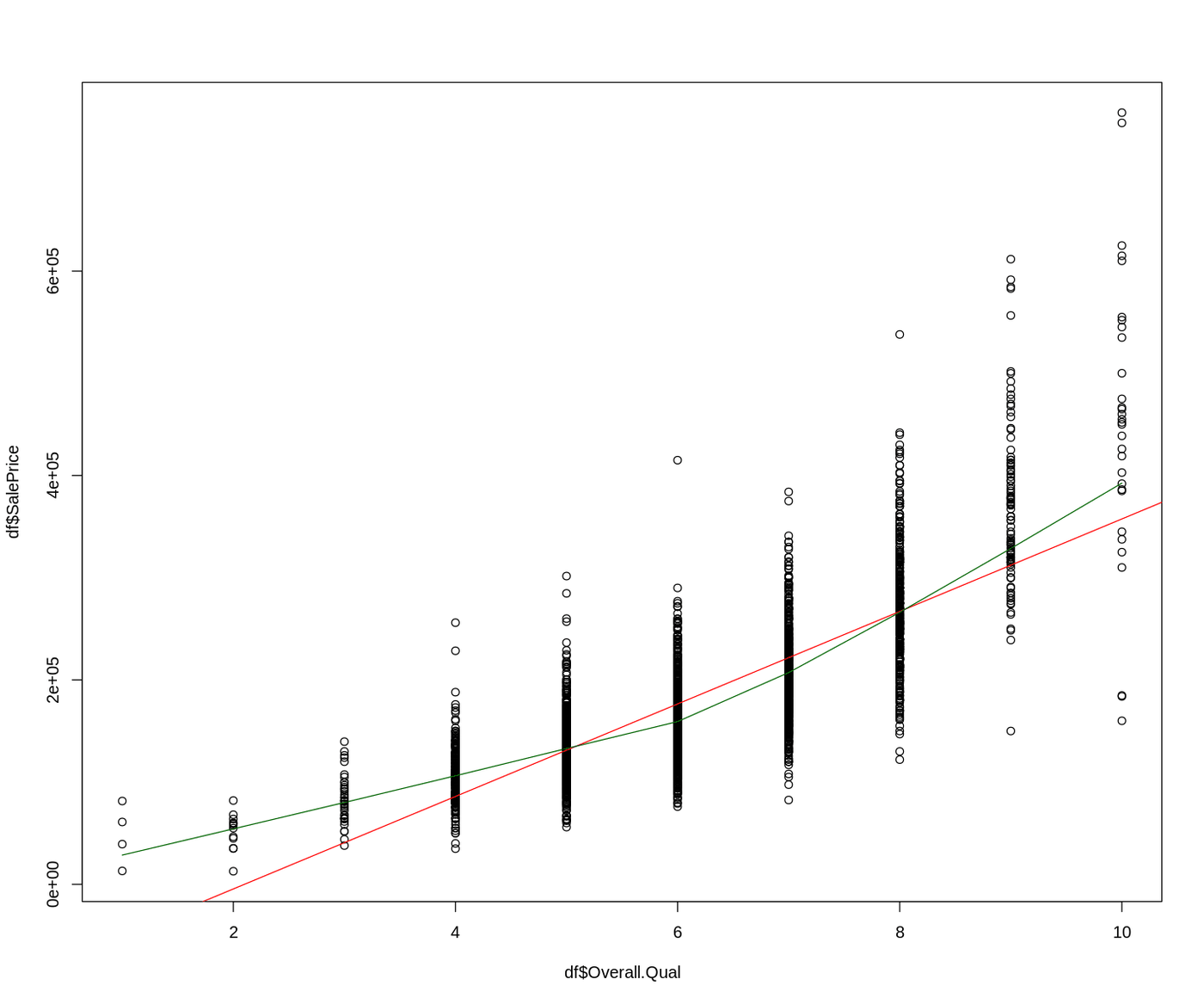
2,930 home sales. kNN imputation, a correlation screen for the top ten drivers, linear to cubic to multiple regression, VIF checks, and ridge regression to remove multicollinearity.

0.64 → 0.70 → 0.80R²: linear, cubic, multiple
2predictors with VIF > 5
kNN imputationlmVIFglmnet ridgeresidual plots
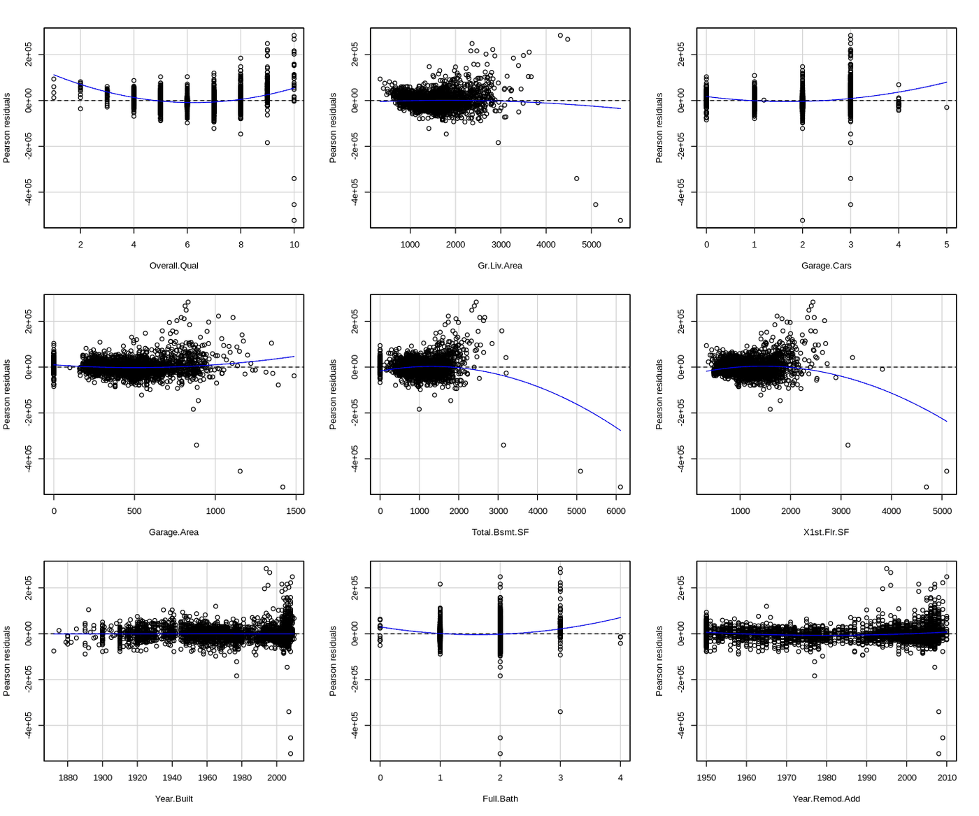
Correlation matrix of the ten predictors most correlated with sale priceSale price by overall quality with linear and LOWESS linesResidual plots for each predictor in the multiple regression
Code · 118 lines
# Ames housing prices: exploratory analysis, kNN imputation, linear and cubic
# models, multiple regression, VIF checks, and ridge regression to handle
# multicollinearity. Data: Ames Housing (2,930 home sales).

library(ggplot2)
library(readr)

df <- read.csv("AmesHousing.csv")

# 1.0 Inspect ----
head(df)
names(df)     # pandas equivalent: df.columns
str(df)       # "structure" in R; closest pandas equivalent is df.info()
# R is data-frame-centric out of the box; Python needs pandas and NumPy for the same structures.

# 2.0 Distribution of sale price ----
summary(df)   # pandas equivalent: df.describe()
summary(df$SalePrice)

Scaled_SalePrice <- df$SalePrice / 1000    # $1k units instead of scientific notation
hist(Scaled_SalePrice, col = "skyblue", xlab = "SalePrice (in 1k units)")
boxplot(Scaled_SalePrice, col = "orange", horizontal = TRUE)
# The box is the middle 50% of prices; the line inside it is the median.
plot(density(Scaled_SalePrice))
# Right-skewed.

# 3.0 Correlations and missing values ----
cor(df$Fireplaces, df$X1st.Flr.SF)   # 0.4, positive

df_numeric <- df[sapply(df, is.numeric)]

# DMwR2 was removed from CRAN, so install it from GitHub instead
devtools::install_github("ltorgo/DMwR2", ref = "master")
library(DMwR2)
df_imputed <- knnImputation(df_numeric, k = 5)
# k-nearest neighbors: to guess a missing grade, ask the 5 classmates with the
# most similar profiles and average their answers.

library(corrplot)
options(repr.plot.width = 12, repr.plot.height = 10)
corrplot(cor(df_imputed), method = "color")

library(skimr)
print(skim(df))
library(DataExplorer)
introduce(df_imputed)
plot_intro(df)
plot_missing(df)

# 4.0 Ten strongest correlations with SalePrice ----
cor_matrix <- cor(df_imputed)
saleprice_cor <- cor_matrix[, "SalePrice"]
# The matrix already holds every pairwise correlation; just pull the SalePrice column.
saleprice_df <- data.frame(Variable = names(saleprice_cor), Correlation = saleprice_cor)
top_10_corr <- saleprice_df[order(-abs(saleprice_df$Correlation)), ][1:10, ]
top_10_corr

# 5.0 SalePrice by overall quality: linear vs cubic ----
df <- df_imputed
plot(df$Overall.Qual, df$SalePrice)
abline(lm(SalePrice ~ Overall.Qual, data = df), col = "red")
lines(lowess(df$Overall.Qual, df$SalePrice), col = "darkgreen")
# The LOWESS curve bends upward, so a curved model should fit better.

model_linear <- lm(SalePrice ~ Overall.Qual, data = df)
summary(model_linear)

# SalePrice = b0 + b1*Qual + b2*Qual^2 + b3*Qual^3 + e
model_cubic <- lm(SalePrice ~ poly(Overall.Qual, 3, raw = TRUE), data = df)
summary(model_cubic)
# The cubic model captures the curvature that the linear model misses.

# 6.0 Multiple regression ----
model_multiple <- lm(SalePrice ~ Overall.Qual +
  Gr.Liv.Area + Garage.Cars + Garage.Area + Total.Bsmt.SF +
  X1st.Flr.SF + Year.Built + Full.Bath + Year.Remod.Add,
  data = df)
summary(model_multiple)

# 7.0 Multicollinearity: correlations above 0.70 and VIF above 5 ----
vars_top10 <- top_10_corr$Variable
cor_top10 <- cor(df[, vars_top10])
corrplot(cor_top10, method = "color", addCoef.col = "black", tl.cex = 0.8)
# High pairs: Garage.Cars / Garage.Area and Total.Bsmt.SF / X1st.Flr.SF

library(car)
vif_values <- vif(model_multiple)
vif_values[vif_values > 5]
# Garage.Area and Total.Bsmt.SF exceed 5. Correlation > 0.70 plus VIF > 5 needs a remedy.

# 8.0 Ridge regression ----
library(glmnet)
X <- model.matrix(SalePrice ~ Overall.Qual + Gr.Liv.Area + Garage.Cars + Garage.Area +
                    Total.Bsmt.SF + X1st.Flr.SF + Year.Built + Full.Bath + Year.Remod.Add,
                  data = df_imputed)[, -1]   # drop the intercept column
y <- df_imputed$SalePrice

set.seed(123)
cv_ridge <- cv.glmnet(X, y, alpha = 0)   # cross-validate lambda
ridge_best_lambda <- glmnet(X, y, alpha = 0, lambda = cv_ridge$lambda.min)
coef(ridge_best_lambda)

# R-squared by hand for the ridge model
y_pred <- predict(ridge_best_lambda, newx = X)
SSE <- sum((y - y_pred)^2)
SST <- sum((y - mean(y))^2)
R2_ridge <- 1 - SSE / SST
R2_ridge
summary(model_multiple)
# Ridge gives up a little predictive power, but the model is more stable and
# free of multicollinearity.

plot(cv_ridge$glmnet.fit, xvar = "lambda")             # coefficient shrinkage paths
abline(v = log(cv_ridge$lambda.min), col = "blue", lty = 2)

# 9.0 Residual check for non-linearity ----
residualPlots(model_multiple)
# Several predictors show patterns (p < 0.05). Fix: transform the target (log or square root).

U.S. Tuition, 2004 to 2016

Tidies a wide state-by-year spreadsheet, joins census regions, and builds charts whose titles state the finding.

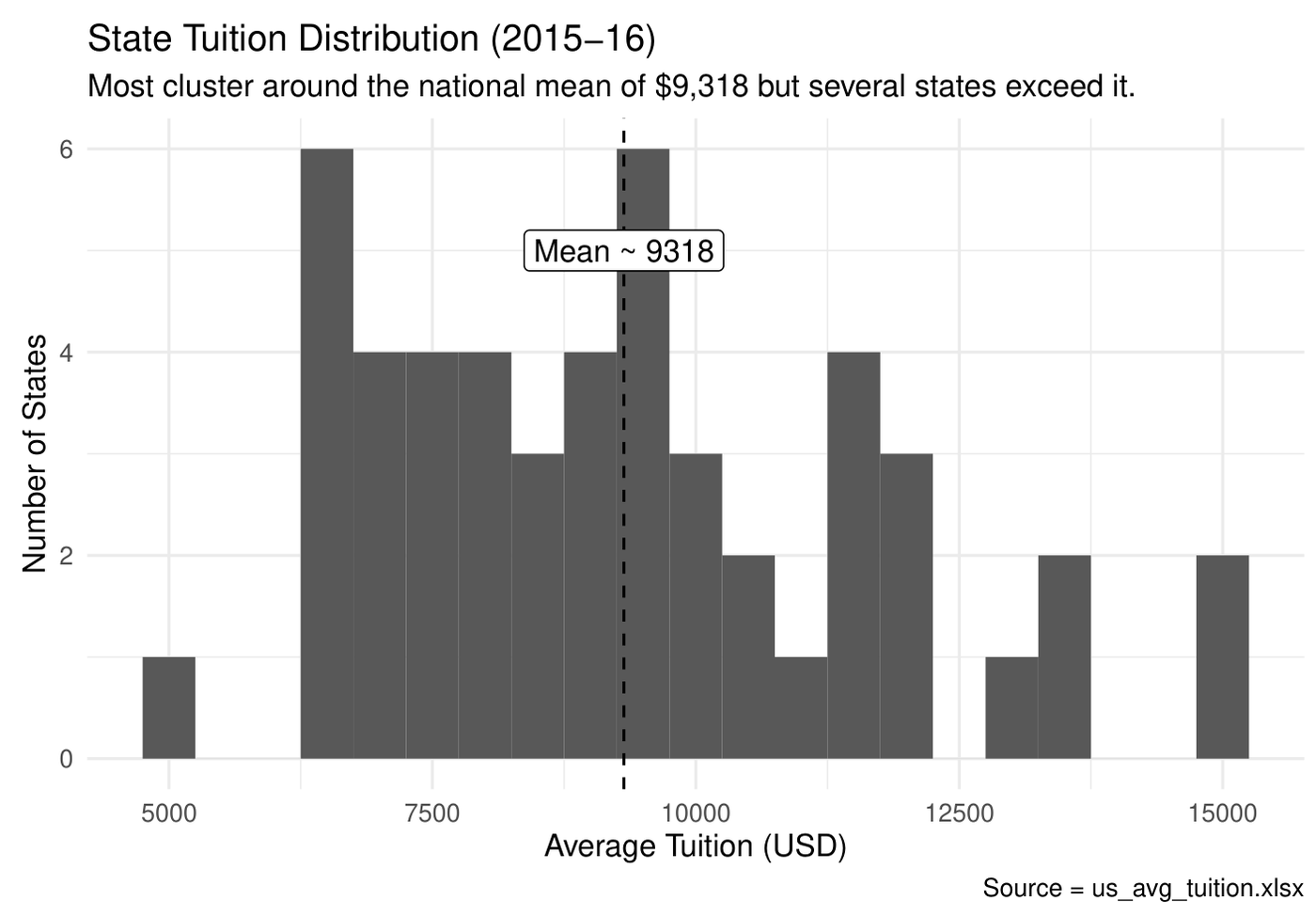
$9,3182015-16 state mean
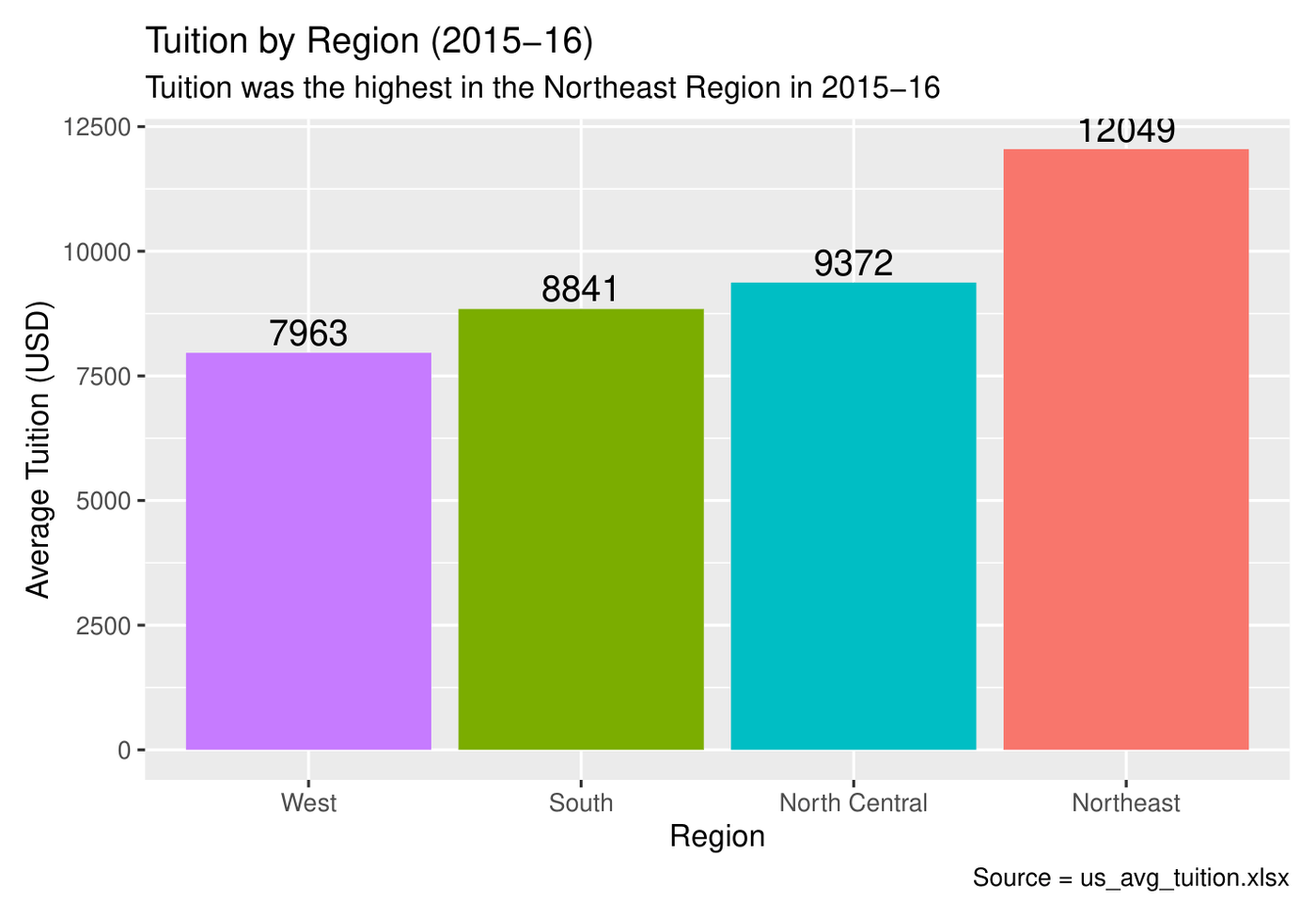
$12,049Northeast, highest region
pivot_longerleft_joinggplot2annotationreference lines
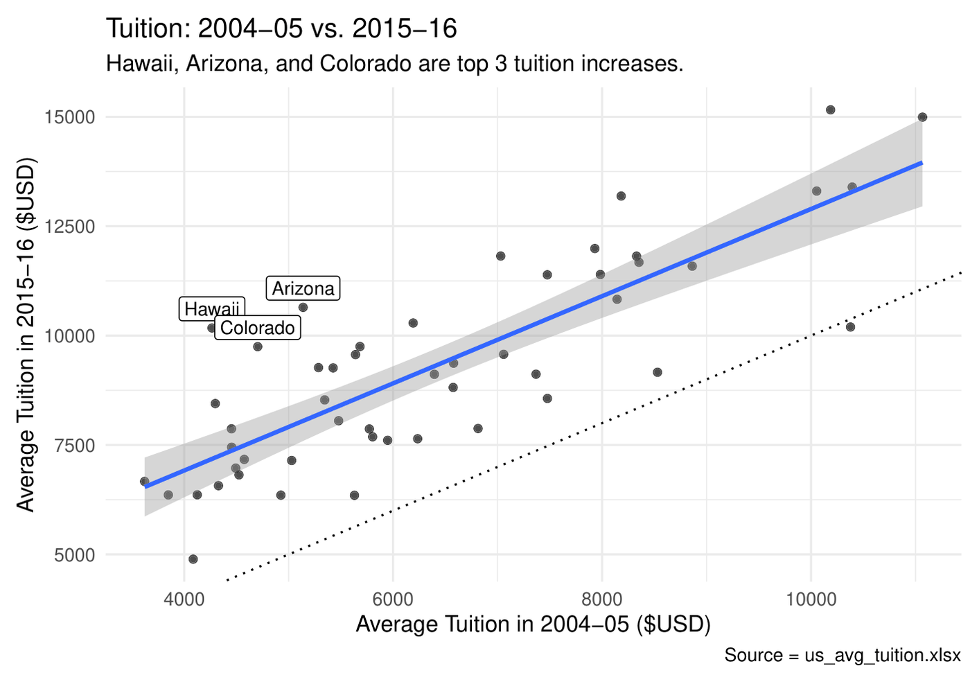
Average tuition by region, 2015-16Distribution of state tuition with mean lineState tuition 2004-05 versus 2015-16
Code · 104 lines
# U.S. college tuition, 2004-05 to 2015-16: tidy a wide spreadsheet, join regions,
# and turn five plain charts into ones that tell the story on their own.
# Data: us_avg_tuition.xlsx (average in-state tuition by state and school year).

library(tidyverse)
library(readxl)

# 1.0 Tidy: one column per year -> one row per state-year ----
us_avg_tuition_raw <- read_excel("us_avg_tuition.xlsx")

state_tuition_long <- us_avg_tuition_raw %>%
  rename_with(tolower) %>%
  pivot_longer(cols = -state, names_to = "school_year", values_to = "avg_cost") %>%
  mutate(
    state = factor(state),
    school_year = as.character(school_year),
    avg_cost = as.numeric(avg_cost)
  )

# Join census regions from R's built-in state data
state_regions <- tibble(state = state.name, region = state.region)
tuition_with_region <- state_tuition_long %>%
  left_join(state_regions, by = "state")

# 2.0 Summaries ----
region_cost_2015 <- tuition_with_region %>%
  filter(school_year == "2015-16") %>%
  group_by(region) %>%
  summarise(avg_cost = mean(avg_cost), .groups = "drop") %>%
  arrange(desc(avg_cost))

national_by_year <- state_tuition_long %>%
  mutate(school_year = factor(school_year, levels = unique(school_year))) %>%
  group_by(school_year) %>%
  summarise(avg_cost = mean(avg_cost), .groups = "drop") %>%
  arrange(school_year)

# 3.0 National trend ----
ggplot(national_by_year, aes(x = school_year, y = avg_cost, group = 1)) +
  geom_line() +
  geom_point() +
  labs(title = "Average U.S. Tuition by Year",
       subtitle = "There is a positive correlation.",
       x = "School Year", y = "Average Tuition (USD)",
       caption = "Source = us_avg_tuition.xlsx") +
  theme(axis.text.x = element_text(angle = 45, hjust = 1))
# Tuition rose steadily from 2004-05 through 2015-16, with the biggest jump
# between 2008-09 and 2009-10. Growth slowed after 2012-13.

# 4.0 Regions, ordered and directly labeled ----
ggplot(region_cost_2015, aes(x = fct_reorder(region, avg_cost), y = avg_cost, fill = region)) +
  geom_col() +
  geom_text(aes(label = round(avg_cost, 0), vjust = -0.3, size = 3)) +
  labs(title = "Tuition by Region (2015-16)",
       subtitle = "Tuition was the highest in the Northeast Region in 2015-16",
       x = "Region", y = "Average Tuition (USD)",
       caption = "Source = us_avg_tuition.xlsx") +
  theme(legend.position = "none")

# 5.0 State distribution with a mean reference line ----
state_2015 <- tuition_with_region %>% filter(school_year == "2015-16")
mean_2015 <- mean(state_2015$avg_cost)

ggplot(state_2015, aes(x = avg_cost)) +
  geom_histogram(binwidth = 500) +
  geom_vline(xintercept = mean_2015, linetype = "dashed") +
  annotate("label", x = mean_2015, y = 5, label = paste0("Mean ~ ", round(mean_2015, 0))) +
  labs(title = "State Tuition Distribution (2015-16)",
       subtitle = "Most cluster around the national mean of $9,318 but several states exceed it.",
       x = "Average Tuition (USD)", y = "Number of States",
       caption = "Source = us_avg_tuition.xlsx") +
  theme_minimal()
# Right-skewed: most states sit near $9,318, a few run much higher.

# 6.0 Spread by region ----
ggplot(state_2015, aes(x = avg_cost, y = region, fill = region)) +
  geom_boxplot() +
  labs(title = "Regional Cost Distribution (2015-16)",
       subtitle = "Northeast has the highest average tuition and widest spread",
       x = "Average Tuition (USD)", y = "Region",
       caption = "Source = us_avg_tuition.xlsx") +
  theme(legend.position = "none")

# 7.0 2004 vs 2015 with a y = x reference and the biggest movers labeled ----
two_years_wide <- tuition_with_region %>%
  filter(school_year %in% c("2004-05", "2015-16")) %>%
  select(state, school_year, avg_cost) %>%
  pivot_wider(names_from = school_year, values_from = avg_cost) %>%
  rename(cost_2004 = `2004-05`, cost_2015 = `2015-16`) %>%
  mutate(delta = cost_2015 - cost_2004)

top3 <- two_years_wide %>% slice_max(delta, n = 3)

ggplot(two_years_wide, aes(x = cost_2004, y = cost_2015)) +
  geom_point(alpha = 0.7) +
  geom_abline(slope = 1, intercept = 0, linetype = "dotted") +
  geom_smooth(method = "lm") +
  geom_label(data = top3, aes(label = as.character(state)), size = 3, vjust = -0.3) +
  labs(title = "Tuition: 2004-05 vs. 2015-16",
       subtitle = "Hawaii, Arizona, and Colorado are top 3 tuition increases.",
       x = "Average Tuition in 2004-05 ($USD)",
       y = "Average Tuition in 2015-16 ($USD)",
       caption = "Source = us_avg_tuition.xlsx") +
  theme_minimal()

120 Years of Olympic Medals

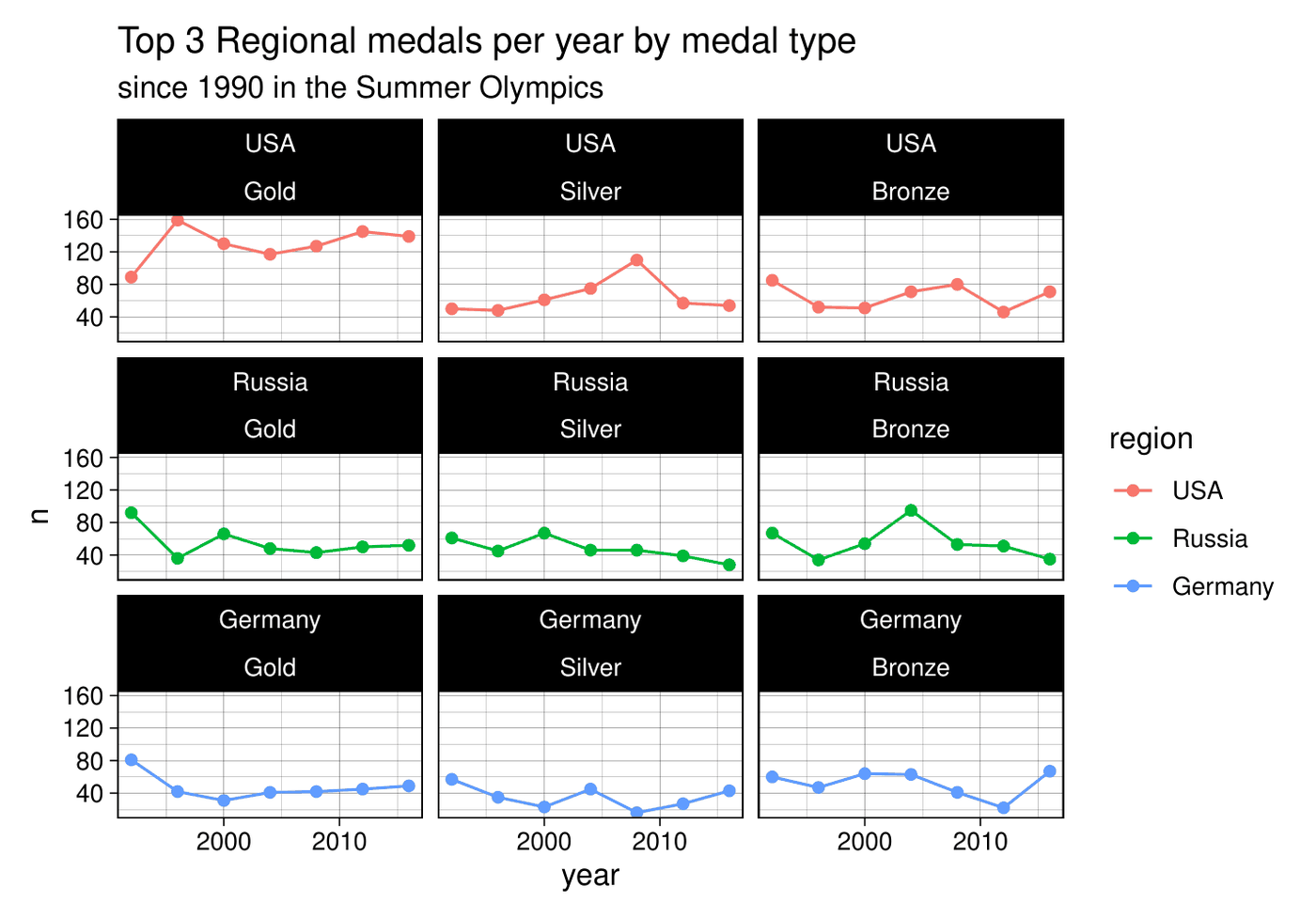
Joins 271,116 athlete-event records to region codes, checks the join before trusting it, and compares the top three regions by medal type since 1990.

271,116athlete-event records
3 × 3region by medal facets
left_joinjoin validationcountfacet_wrap
Medals per Summer Games for USA, Russia and Germany by medal type
Code · 67 lines
# 120 years of Olympic results: join country codes to regions, validate the
# join, rank regions by medals, and compare the leaders with faceted trends.
# Data: 271,116 athlete-event records (1896-2016) and 206 NOC region codes.

library(tidyverse)

olympic_events_raw <- read_csv("olympic_history_athlete_events.csv")
noc_regions <- read_csv("olympic_history_noc_regions.csv")

# 1.0 Join and keep medal winners only ----
olympic_events <- olympic_events_raw %>%
  left_join(noc_regions, by = 'NOC') %>%
  rename_with(tolower) %>%
  filter(!is.na(medal))

# Validate the join before trusting it
sum(is.na(olympic_events$medal)) == 0
sum(is.na(olympic_events$region)) == 0
ncol(olympic_events) == (ncol(olympic_events_raw) + ncol(noc_regions %>% select(-region)))

# 2.0 Which region leads each medal type in the Summer Games? ----
region_medal_count <- olympic_events %>%
  filter(season == "Summer") %>%
  count(region, medal, sort = TRUE)

region_medal_count %>% filter(medal == "Gold")   %>% top_n(1) %>% .$region
region_medal_count %>% filter(medal == "Silver") %>% top_n(1) %>% .$region
region_medal_count %>% filter(medal == "Bronze") %>% top_n(1) %>% .$region

# 3.0 Top six regions since 1990 ----
top_6 <- olympic_events %>%
  filter(season == "Summer") %>%
  count(region, sort = TRUE) %>%
  top_n(6)

olympic_top6 <- olympic_events %>%
  filter(season == "Summer", year >= 1990, region %in% top_6$region)

olympic_top6 %>%
  count(year, region) %>%
  ggplot(aes(x = year, y = n, color = region)) +
  geom_point() +
  geom_line() +
  ggtitle("Top 6 Regional medals per year", "since 1990 in the Summer Olympics") +
  theme_minimal()
# The United States has led every region in Summer medals since 1990, with a peak in 2008.

# 4.0 Top three regions, split by medal type ----
top_3 <- olympic_events %>%
  filter(season == "Summer") %>%
  count(region, sort = TRUE) %>%
  top_n(3)

olympic_top3_ordered <- olympic_events %>%
  filter(season == "Summer", year >= 1990, region %in% top_3$region) %>%
  mutate(medal = factor(medal, levels = c("Gold", "Silver", "Bronze")),
         region = factor(region, levels = top_3$region))

olympic_top3_ordered %>%
  count(year, region, medal) %>%
  ggplot(aes(x = year, y = n, color = region)) +
  geom_point() +
  geom_line() +
  ggtitle("Top 3 Regional medals per year by medal type", "since 1990 in the Summer Olympics") +
  facet_wrap(region ~ medal, ncol = 3) +
  theme_linedraw()
# The United States wins the most medals in every category at every Summer Games since 1990.

U.S. Milk Production

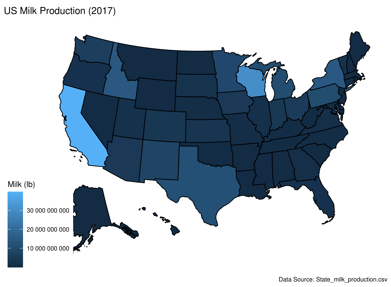
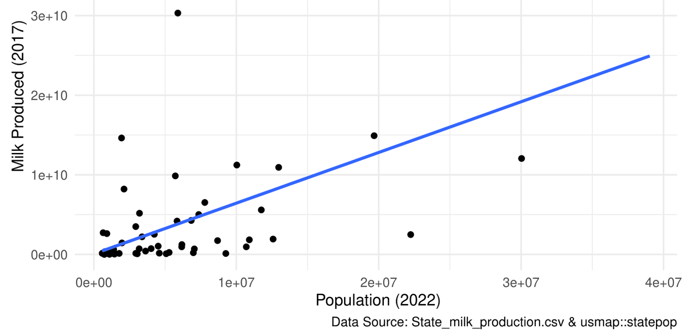
Reads 1970-2017 state data straight from the web, maps 2017 output, and joins population to test whether bigger states produce more milk.

r = 0.63population vs milk produced
read from URLusmapleft_joincor
Choropleth map of 2017 milk productionState population versus milk produced
Code · 74 lines
# U.S. milk production 1970-2017: pull data straight from the web, map it by
# state, then join population data and test the relationship.
# Data: TidyTuesday state milk production (2019-01-29) and usmap::statepop.

library(tidyverse)
library(usmap)

milk_production_data <- read.csv(
  "https://raw.githubusercontent.com/rfordatascience/tidytuesday/master/data/2019/2019-01-29/state_milk_production.csv"
)

# 1.0 Profile the data ----
q1_year_min <- summarise(milk_production_data, min(year)) %>% pull()
q1_year_max <- summarise(milk_production_data, max(year)) %>% pull()

q2_state_count <- milk_production_data %>%
  summarise(n_states = n_distinct(state)) %>%
  pull()
q2_has_50_states <- (q2_state_count == 50)

q3_top_state_2017 <- milk_production_data %>%
  filter(year == 2017) %>%
  arrange(desc(milk_produced)) %>%
  slice(1) %>%
  pull(state)

# 2.0 Production over time by region ----
ggplot(milk_production_data, aes(x = year, y = milk_produced, color = region)) +
  geom_point() +
  labs(title = "Milk Production by US state over time",
       x = "Year", y = "Milk Produced (lb)", color = "Region",
       caption = "Data Source: State_milk_production.csv") +
  theme_minimal()
# Shows consistent regional differences and the long-run trend from 1970 to 2017.

# 3.0 Choropleth map, 2017 ----
milk_2017 <- milk_production_data %>%
  filter(year == 2017) %>%
  select(state, milk_produced)

plot_usmap(data = milk_2017, values = "milk_produced", color = "black") +
  scale_fill_continuous(name = "Milk (lb)", labels = scales::label_number()) +
  labs(title = "US Milk Production (2017)",
       caption = "Data Source: State_milk_production.csv")
# Totals are not normalized by population, so read this as volume, not per-capita production.

# 4.0 Does population track production? ----
statepop_renamed <- usmap::statepop %>% rename(state = full)

# Find the most recent population column without hard-coding its name
pop_recent_col <- grep("pop_", names(statepop_renamed), value = TRUE)
pop_recent_yr <- gsub("pop_", "", pop_recent_col)

milk_recent <- milk_production_data %>%
  filter(year == q1_year_max) %>%
  select(state, milk_produced)

milk_pop_recent <- left_join(milk_recent, statepop_renamed, by = "state")

r_pop_milk <- cor(milk_pop_recent[[pop_recent_col]],
                  milk_pop_recent$milk_produced,
                  use = "complete.obs")

ggplot(milk_pop_recent, aes(x = .data[[pop_recent_col]], y = milk_produced)) +
  geom_point() +
  geom_smooth(method = "lm", se = FALSE) +
  labs(title = paste0("Population vs. Milk Production (", q1_year_max, ")"),
       subtitle = "Population and milk production are positively correlated (r = 0.63)",
       x = paste0("Population (", pop_recent_yr, ")"),
       y = paste0("Milk Produced (", q1_year_max, ")"),
       caption = "Data Source: State_milk_production.csv & usmap::statepop") +
  theme_minimal()
# Population is from 2022 and milk from 2017, so treat population as an indicator,
# not an exact match. r = 0.63: larger states tend to produce more milk.

Foundations

R fundamentalsVectors to data frames, NA-safe derived columns, and small functions that chain with the pipe. · 58 lines
# R fundamentals: vectors and data frames, subsetting, derived columns,
# and writing small reusable functions that chain with the pipe.

library(tidyverse)

# 1.0 Build a data frame from vectors ----
name_vector   <- c("Jake", "Pepsi", "Laura", "James", "Ron", "Spencer")
score_vector  <- c(NA, 70, 95, 90, 86, 77)
passed_vector <- c(FALSE, FALSE, TRUE, TRUE, TRUE, FALSE)

df <- data.frame(name = name_vector,
                 score = score_vector,
                 passed = passed_vector,
                 stringsAsFactors = FALSE)

# 2.0 Subset by position and by condition ----
part_a <- df[2:5, c("name", "score")]
score_85_condition <- df$score >= 85
part_b <- df[score_85_condition, c("name", "score")]

# 3.0 Derived columns: z-score and letter grade, NA-safe ----
df$z_score <- (df$score - mean(df$score, na.rm = TRUE)) / sd(df$score, na.rm = TRUE)

df$grade_band <- ifelse(
  is.na(df$score), NA,
  ifelse(df$score >= 90, "A",
  ifelse(df$score >= 80 & df$score <= 89, "B",
  ifelse(df$score >= 70 & df$score <= 79, "C",
  ifelse(df$score >= 60 & df$score <= 69, "D", "F")))))

cat("Mean:", mean(df$score, na.rm = TRUE), "\n")
cat("SD:",   sd(df$score,   na.rm = TRUE), "\n")
cat("Min:",  min(df$score,  na.rm = TRUE), "\n")
cat("Max:",  max(df$score,  na.rm = TRUE), "\n")

# 4.0 Functions ----
head_func2 <- function(df, n = 6) {
  if (n <= 0) {
    result <- df[0, ]          # zero rows, same columns
  } else {
    result <- df[1:n, ]
  }
  return(result)
}

select_make_model_year <- function(df) {
  df %>% select(manufacturer, model, year)
}

filter_manufacturer <- function(df, manufacturer_name) {
  df %>% filter(manufacturer == manufacturer_name)
}

# Custom functions drop straight into a pipe
land_rover_models <- mpg %>%
  select_make_model_year() %>%
  filter_manufacturer("land rover") %>%
  arrange(year)