Jake Moore | Python

Bike Sales: From Three Tables to a Revenue Trend

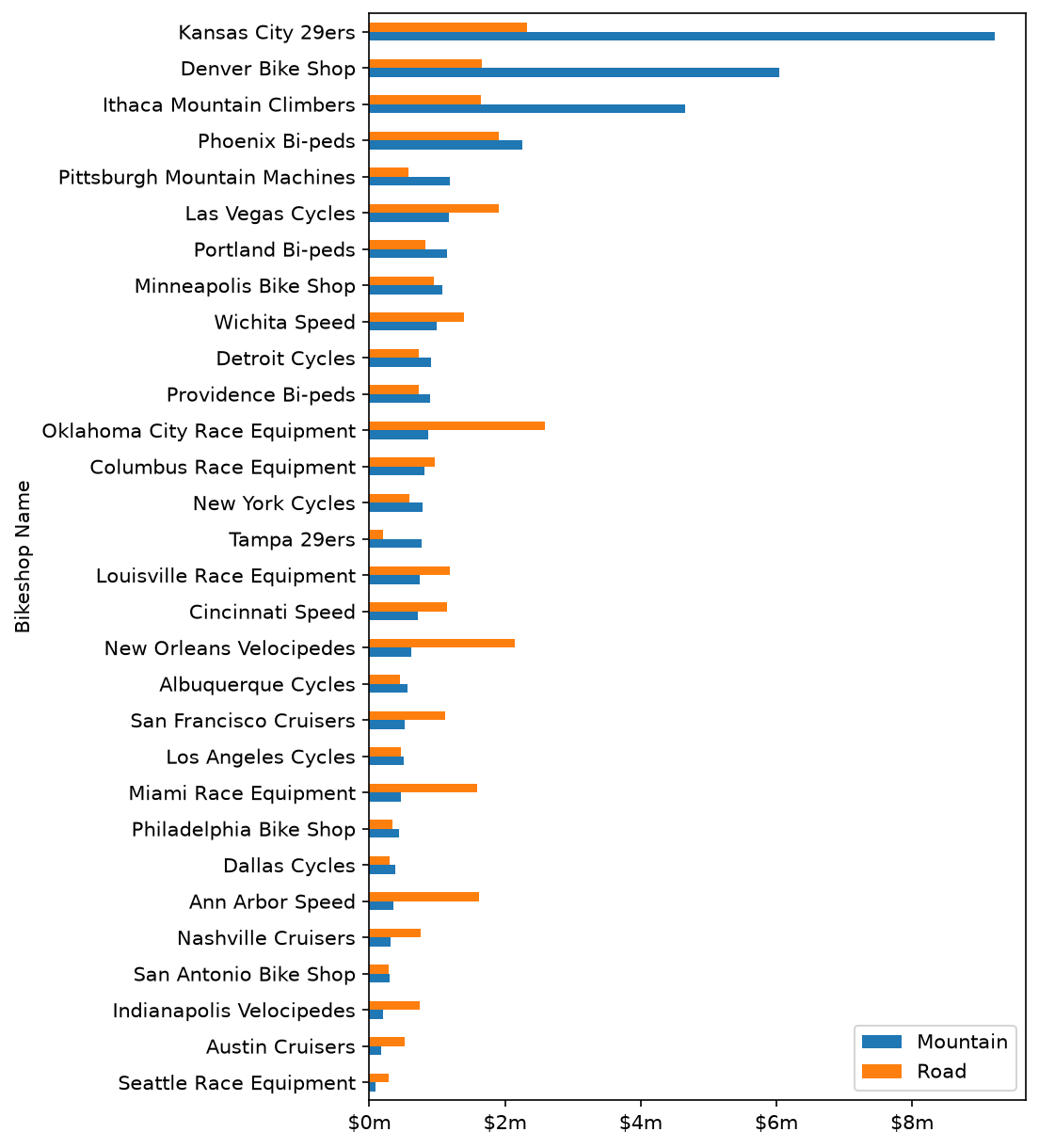
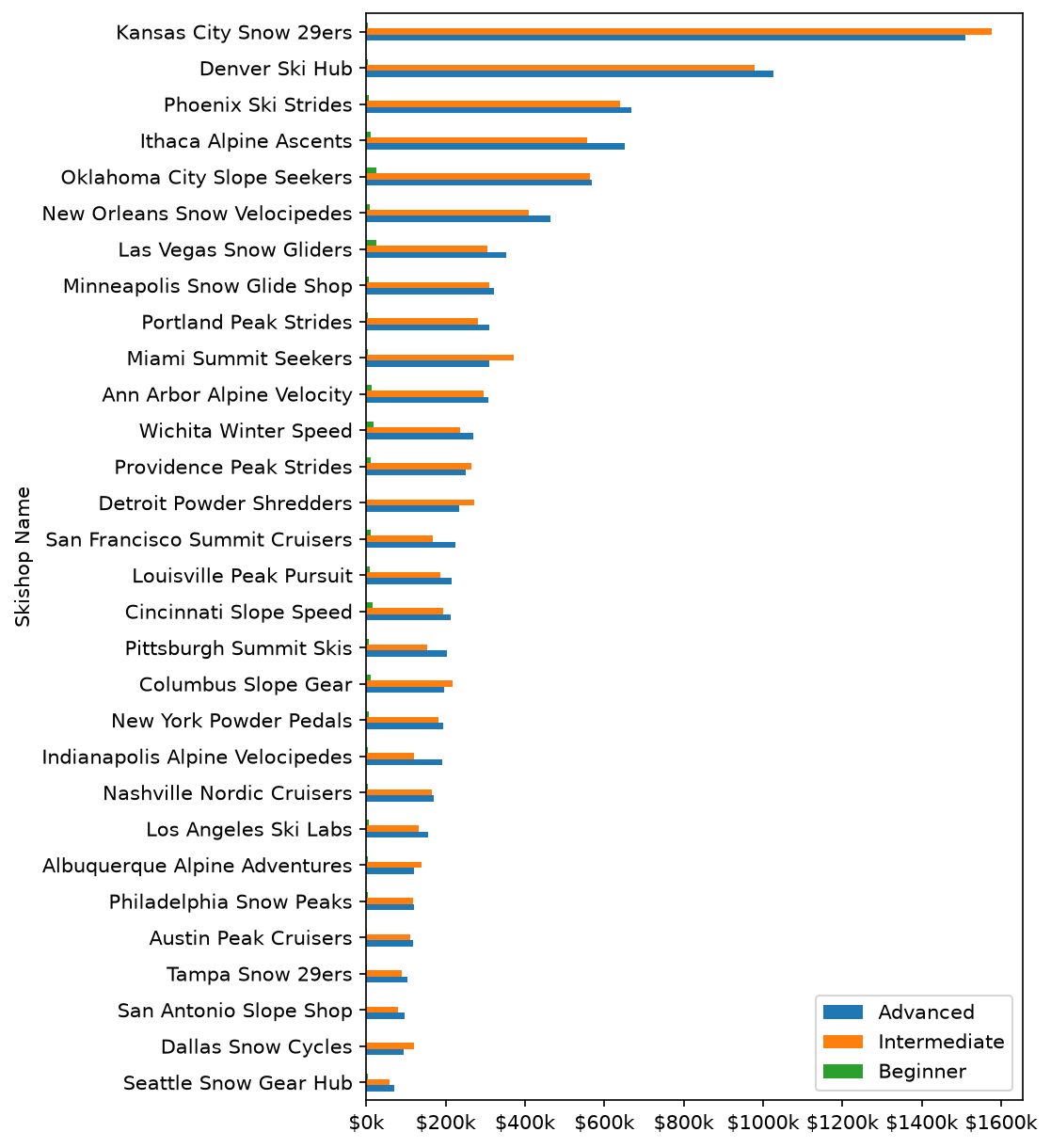
Joins 15,644 order lines to 97 bike models and 30 shops, splits product and location text into usable columns, and rolls revenue up by month and by week for each sub-category.

15,644order lines joined

9sub-categories tracked weekly

mergemethod chainingstr.splitresampleplotnine

Monthly bike revenue 2011 to 2015 with a LOWESS trend line

Weekly revenue panels for each bike sub-category

Code · 110 lines

# Bike sales pipeline: join three tables, clean text fields, build revenue,
# then roll orders up to monthly and weekly revenue trends.
# Data: bikes.xlsx, bikeshops.xlsx, orderlines.xlsx (15,644 order lines, 97 bikes, 30 shops)

import pandas as pd
import numpy as np
import matplotlib.pyplot as plt
from mizani.formatters import currency_format
from plotnine import (
    ggplot, aes,
    geom_line, geom_smooth,
    scale_y_continuous,
    labs, theme_minimal, expand_limits,
)

# 1.0 Read the three source tables
bikes_df = pd.read_excel("bikes.xlsx")
bikeshop_df = pd.read_excel("bikeshops.xlsx")
orderlines_df = pd.read_excel("orderlines.xlsx")

# 2.0 Quick look: five best-selling bike descriptions
top5_bike_series = bikes_df['description'].value_counts().nlargest(5)
top5_bike_series.plot(kind="barh", color="black")
plt.show()

# 3.0 Join order lines to products and shops in one method chain
bike_orderlines_joined_df = orderlines_df \
    .drop(columns='Unnamed: 0') \
    .merge(
        right=bikes_df,
        how='left',
        left_on='product.id',
        right_on='bike.id'
    ) \
    .merge(
        right=bikeshop_df,
        how='left',
        left_on='customer.id',
        right_on='bikeshop.id'
    )

# 4.0 Split compound text fields into their own columns
df = bike_orderlines_joined_df.copy()

# "Road - Elite Road - Carbon" -> category, sub-category, material
temp_df = df['description'].str.split(" - ", expand=True)
df['Category_1'] = temp_df[0]
df['Category_2'] = temp_df[1]
df['Material'] = temp_df[2]

# "Ithaca, NY" -> city, state
temp_df = df['location'].str.split(", ", expand=True)
df['City'] = temp_df[0]
df['State'] = temp_df[1]

# 5.0 Extended price, then keep only the columns the analysis needs
df['total_revenue'] = df['price'] * df['quantity']
df.sort_values('total_revenue', ascending=False).head(10)

cols_to_keep_list = [
    'order.id', 'order.line', 'order.date', 'quantity',
    'bike.id', 'model', 'description', 'price',
    'bikeshop.id', 'bikeshop.name', 'location',
    'Category_1', 'Category_2', 'Material', 'City',
    'total_revenue',
]
df = df[cols_to_keep_list].copy()

# Dots in column names break attribute access, so swap them for underscores
df.columns = df.columns.str.replace(".", "_")

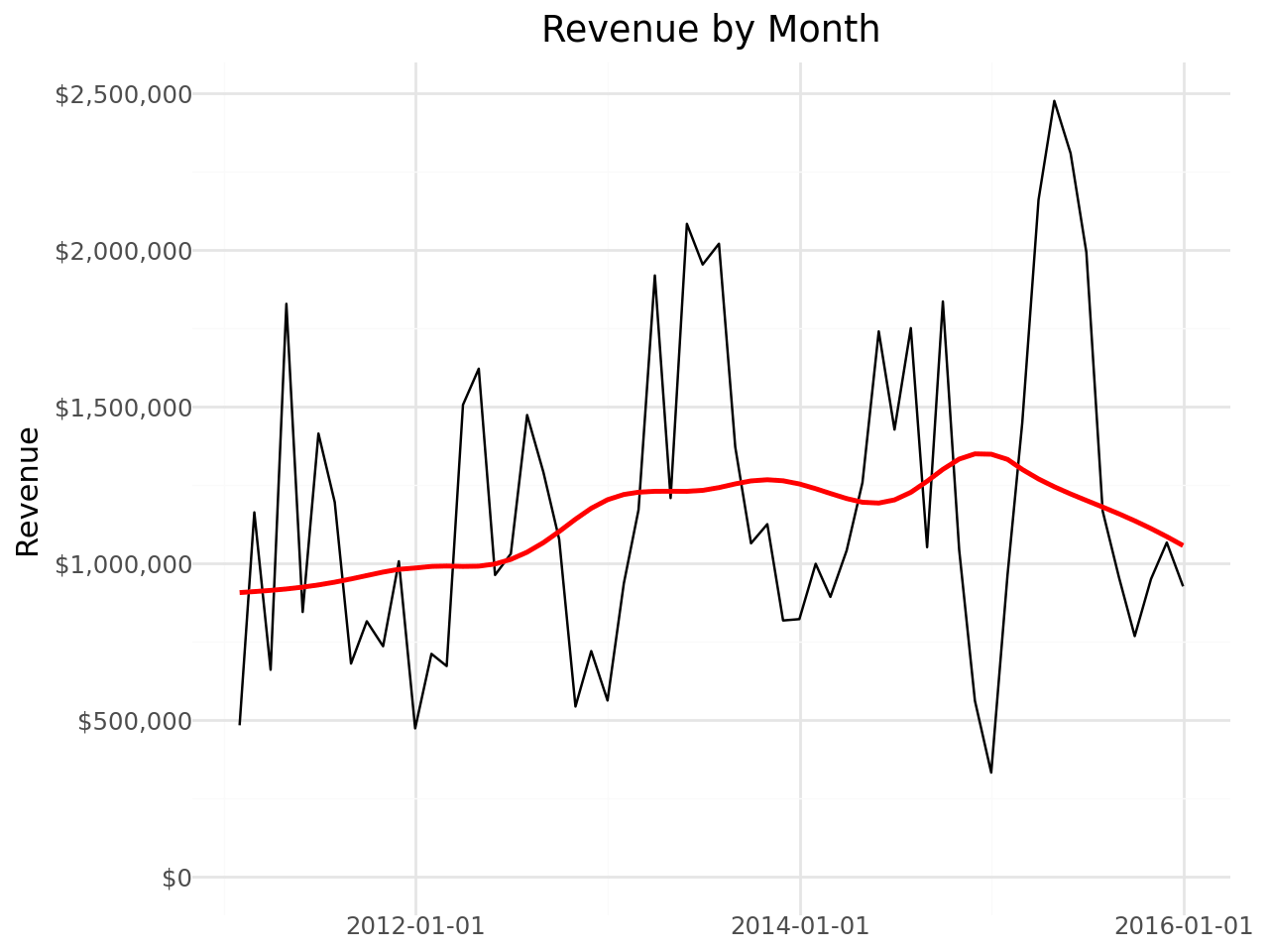
# 6.0 Monthly revenue trend
# Time series order of operations:
#   set the date column as the index -> group -> resample -> aggregate
sales_month_df = df[["order_date", "total_revenue"]] \
    .set_index("order_date") \
    .resample(rule="MS") \
    .aggregate(np.sum) \
    .reset_index()

usd = currency_format(prefix="$", precision=0, big_mark=",")

(
    ggplot(data=sales_month_df, mapping=aes(x="order_date", y="total_revenue"))
    + geom_line()
    + geom_smooth(method='lowess', color='red', span=0.4, se=True)
    + scale_y_continuous(labels=usd)
    + labs(title='Revenue by Month', x='', y='Revenue')
    + theme_minimal()
    + expand_limits(y=10)
)

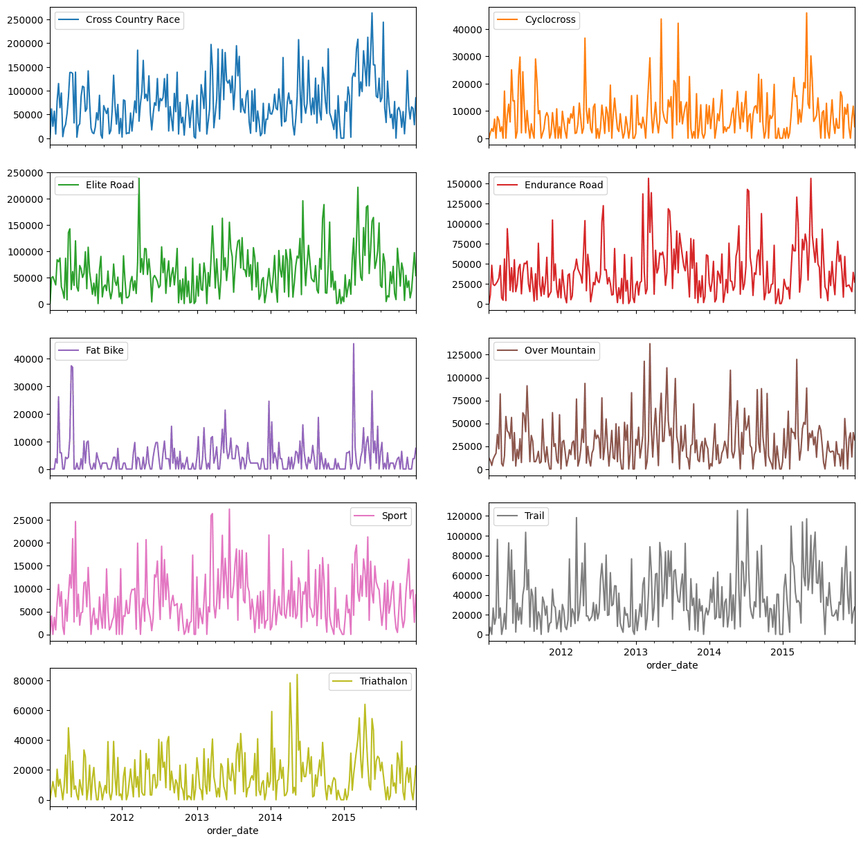
# 6.2 Weekly revenue for each sub-category
sales_by_level_week = df[['Category_2', 'order_date', 'total_revenue']] \
    .set_index('order_date') \
    .groupby('Category_2') \
    .resample("W") \
    .agg(np.sum) \
    .drop(columns='Category_2') \
    .reset_index()

# Long -> wide so each sub-category gets its own panel
sales_by_level_week \
    .pivot(
        index="order_date",
        columns="Category_2",
        values="total_revenue"
    ) \
    .fillna(0) \
    .plot(kind="line", subplots=True, layout=(5, 2), figsize=(15, 15))

Which Shops Sell What: Group, Pivot, Compare

Totals revenue by shop and product line, pivots long to wide, and plots each shop's mix side by side.

30shops compared per dataset

Kansas Citytop revenue in both datasets

groupbyaggpivotlambda renamematplotlib

Revenue by bike shop, mountain versus road

Revenue by ski shop for advanced, intermediate and beginner products

Code · 81 lines

# Aggregate revenue by shop and product line, reshape long -> wide,
# and plot a formatted comparison chart. Same pattern on two datasets.

import pandas as pd
import numpy as np
from matplotlib.ticker import FuncFormatter

# 1.0 Ski shops: revenue by shop and skill level
df = pd.read_pickle("ski_orderlines_wrangled_df.pkl")

# Sum and median revenue per level
df[['Level', 'total_revenue']] \
    .groupby(['Level']) \
    .agg([np.sum, np.median]) \
    .reset_index()

# Total revenue by shop and level, sorted, with readable column names
skishop_revenue_df = df[['skishop_name', 'Level', 'total_revenue']] \
    .groupby(['skishop_name', 'Level']) \
    .agg(np.sum) \
    .reset_index() \
    .sort_values('total_revenue', ascending=False) \
    .rename(columns=lambda x: x.replace("_", " ").title())

# Long -> wide: one row per shop, one column per level
skishop_revenue_wide_df = skishop_revenue_df \
    .pivot(
        index='Skishop Name',
        columns='Level',
        values='Total Revenue'
    ) \
    .reset_index()
skishop_revenue_wide_df.columns = ['Skishop Name', 'Advanced', 'Beginner', 'Intermediate']

skishop_revenue_wide_df \
    .sort_values("Advanced") \
    .plot(
        x="Skishop Name",
        y=["Advanced", "Intermediate", "Beginner"],
        kind="barh",
        figsize=(6, 10)
    ) \
    .xaxis.set_major_formatter(FuncFormatter(
        lambda x, pos: f'${int(x/1000)}k'     # 125000 -> $125k
    ))

# 2.0 Bike shops: same pattern, mountain vs road
df = pd.read_pickle("bike_orderlines_wrangled_df.pkl")

df[['category_1', 'category_2', 'total_price']] \
    .groupby(['category_1', 'category_2']) \
    .agg([np.sum, np.mean]) \
    .reset_index()

bike_price_df = df[['bikeshop_name', 'category_1', 'total_price']] \
    .groupby(['bikeshop_name', 'category_1']) \
    .agg(np.sum) \
    .reset_index() \
    .sort_values('total_price', ascending=False) \
    .rename(columns=lambda x: x.replace('_', ' ').title())

bike_price_wide_df = bike_price_df \
    .pivot(
        index='Bikeshop Name',
        columns='Category 1',
        values='Total Price'
    ) \
    .reset_index()
bike_price_wide_df.columns = ['Bikeshop Name', 'Mountain', 'Road']

bike_price_wide_df \
    .sort_values('Mountain') \
    .plot(
        x='Bikeshop Name',
        y=['Mountain', 'Road'],
        kind='barh',
        figsize=(6, 10)
    ) \
    .xaxis.set_major_formatter(FuncFormatter(
        lambda x, pos: f'${int(x/1000000)}m'  # millions this time
    ))

Will a Subscriber Buy? XGBoost Classifier

Trains a gradient-boosted classifier on 19,900 email subscribers (80/20 split, 10-fold cross-validation) from member rating and country, then scores a new subscriber.

17.6%purchase probability, rating 5, U.S.

10-foldcross-validation

PyCaretXGBoosttrain/test splitcross-validation

predict_model(xgb_model_finalized, new_df, raw_score=True) member_rating country_code prediction_score_0 prediction_score_1 5 us 0.8239 0.1761

Code · 50 lines

# Predict whether an email subscriber will make a purchase, using an
# XGBoost classifier trained and cross-validated through PyCaret.
# Data: subscribers joined with purchase history (about 19,900 rows).

import pandas as pd
import pycaret.classification as clf

subscribers_joined_df = pd.read_pickle("subscribers_joined_df.pkl")

# 1.0 Features and target
df = subscribers_joined_df[["member_rating", "country_code", "made_purchase"]]
# member_rating = numeric feature, country_code = categorical feature

# 2.0 Set up the experiment: 80/20 train-test split, fixed seed
clf_1 = clf.setup(
    data=df,
    target="made_purchase",
    train_size=0.8,
    session_id=123
)
# Binary target; transformed train set shape (15920, 3)

# 3.0 Train XGBoost (Extreme Gradient Boosting)
# Think of friends guessing someone's age. Averaging many guesses beats any
# single guess. Boosting goes further: each friend sees the earlier guesses
# and corrects them, so the combined guess keeps getting closer.
xgb_model = clf.create_model(estimator="xgboost")
# 10-fold cross-validation.
# AUC: 0.5 = random guessing, 1.0 = perfect.

# 4.0 Retrain on all of the data
xgb_model_finalized = clf.finalize_model(xgb_model)

# 5.0 Score a new subscriber: rating 5, United States
new_df = pd.DataFrame(dict(
    member_rating=[5],
    country_code=["us"],
))

clf.predict_model(
    estimator=xgb_model_finalized,
    data=new_df,
    raw_score=True
)
# prediction_score_0 = 0.8239, prediction_score_1 = 0.1761
# -> about an 18% chance this subscriber buys

# 6.0 Save and reload the model
clf.save_model(model=xgb_model_finalized, model_name="xgb_model_finalized")
clf.load_model(model_name="xgb_model_finalized")

Foundations

Selecting and filteringColumns by name, position, regex and type; rows by masks, query strings and seeded samples. · 64 lines

# Selecting columns and filtering rows in pandas: by name, position, regex,
# data type, boolean masks, query strings, slicing and reproducible sampling.
# Data: ski order lines (12,947 rows).

import pandas as pd

df = pd.read_pickle("ski_orderlines_wrangled_df.pkl")

# 1.0 Select by name
df[['order_date', 'order_id', 'order_line']]
df['order_date']        # one bracket  -> Series (1-D)
df[['order_date']]      # two brackets -> DataFrame (2-D)

# 2.0 Select by position
df.iloc[:, 0:3]         # first 3 columns, ":" = all rows
df.iloc[:, -3:]         # last 3 columns, negative indexing

# 3.0 Select by text matching (regex)
#   'term'  contains      '^term' starts with
#   'term$' ends with     (a)|(b) a OR b
# Closer to Excel's REGEXMATCH than to MATCH.
df.filter(regex='(^model)|(^Level)', axis=1)
df.filter(regex='(price$)|(date$)', axis=1)

# 4.0 Rearranging columns
# Single column to the front
l = df.columns.tolist()
l.remove('model')
df[['model', *l]]        # *l unpacks the list

# Several columns to the front with a list comprehension
cols_to_front = ['model', 'Level']
l2 = [col for col in df.columns.tolist() if col not in cols_to_front]
df[[*cols_to_front, *l2]]

# 5.0 Select by data type
df1 = df.select_dtypes(include='object')
df2 = df.select_dtypes(exclude='object')
pd.concat([df1, df2], axis=1)
# concat needs intermediate frames; the list comprehension above does not,
# so it is the lighter option on memory.

# 6.0 Row filters with boolean masks
df.order_date >= pd.to_datetime('2015-01-01')        # boolean Series
df[df.order_date >= pd.to_datetime('2015-01-01')]    # apply the mask
df[df['model'] == 'Nitro Dropout']
df[df['model'].str.startswith('Never')]
df[df['model'].str.contains('Proto Type')]

# 7.0 query(): string filters that read cleanly inside a method chain
price_threshold_1 = 1600
price_threshold_2 = 700
df.query('(price >= @price_threshold_1) | (price <= @price_threshold_2)')
df.query(f'price >= {price_threshold_1}')   # works, but @variables are cleaner

# 8.0 Slicing
df[:5]
df.head(5)
df.tail(5)
df.iloc[0:5, [1, 3, 5]]   # loc = by label, iloc = by position

# 9.0 Sampling, e.g. for train/test splits
df.sample(n=10, random_state=123)       # random_state makes it reproducible
df.sample(frac=0.10, random_state=123)

How pandas is builtDataFrame to Series to NumPy array, plus dictionaries, lists and type casting. · 78 lines

# How pandas is built: objects, classes, and the structures underneath a DataFrame.
# Data: ski order lines (12,947 rows x 13 columns), already joined and cleaned.

import pandas as pd
import numpy as np

df = pd.read_pickle("ski_orderlines_wrangled_df.pkl")

# 1.0 Everything is an object
type(df)
# pandas.core.frame.DataFrame
# An object bundles
#   attributes (data, indexes, columns)
#   methods (groupby, agg, reset_index)

type(df).__mro__
# Method Resolution Order: most specific class first, most generic last
#   (DataFrame, NDFrame, PandasObject, DirNamesMixin, IndexingMixin, OpsMixin, object)

type("car").mro()
# [str, object]

df.shape
# (12947, 13)

df.query("Level == 'Intermediate'")
# A method is a function attached to an object

# 2.0 The three layers of a DataFrame
type(df['order_date'])
# pandas.core.series.Series -> each column is a Series

df['order_date'].dt.year
# .dt is an accessor, like .str: it reaches inside the Series

type(df.index)

type(df['order_date'].values).mro()
# [numpy.ndarray, object]
# Externally order_date is a pandas Series; internally it is a NumPy array.
#
#   1) DataFrame   holds many Series
#   2) Series      adds an index and a name
#   3) NumPy array does the fast math (sum, mean, std, log) in C

# 3.0 Core Python structures
# Dictionaries: key-value pairs with fast lookup.
# Used constantly in pandas: df.rename(), df.agg(), and **kwargs are all dictionaries.
d = {'a': 1}
type(d)          # dict
d.keys()         # dict_keys(['a'])
d.values()       # dict_values([1])
d['a']           # 1

# Lists: ordered collections, the workhorse of loops
l = [1, 'A', [2, 'B']]   # integer, string, nested list
l[0]
l[1]
l[2]
list(d.values())[0]

# Base types: str, int, float, bool
type(1.5).mro()
type(1)
df.total_revenue.values            # array([ 890, 1230,  700, ..., 1670, 1190, 1520])
type(df['model'].values[0])        # str

# 4.0 Casting: converting between types, the heart of data cleaning
model = 'Rossignol'
price = 6070
f'The first model is {model}'
f'The price of the first model is {price}'
str(price) + 'USD'
str(1.0)
int('50%'.replace('%', ''))        # "50%" -> 50

r = list(range(1, 51))
r_array = np.array(r)              # list -> NumPy array for fast vector math